

For the best experience,
browse Cellestial website on a computer.
Cellestial v0.60.0#




The grammar of graphics for single-cell omics.
Installation#
pip install cellestial
uv add cellestial
poetry add cellestial
Examples#
Hover over the plot ‘geoms’ to see tooltips, or use toolbar above the plot for zooming and panning options.
Spatial#
Overlay categorical labels or gene expression on tissue coordinates.
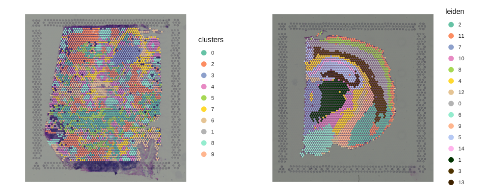
Show code
import cellestial as cl
import squidpy as sq
from ggrust import *
data_spatial = cl.datasets.human_lymph_node()
data_hne = sq.datasets.visium_hne_adata()
s1 = cl.spatial(data_spatial, key="clusters")
s2 = cl.spatial(data_hne, key="leiden")
spatial_categorical = gggrid([s1, s2], ncol=2) + ggsize(1000, 400) + ggtb(size_zoomin=-1)
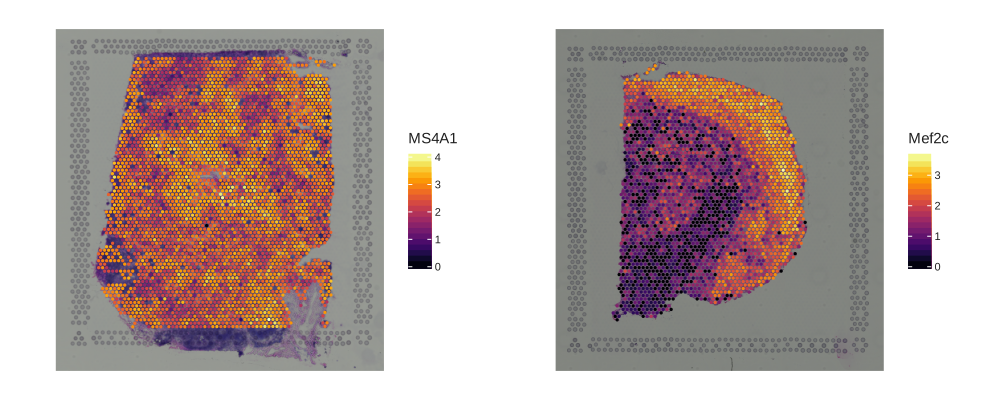
Show code
import cellestial as cl
import squidpy as sq
from ggrust import *
data_spatial = cl.datasets.human_lymph_node()
data_hne = sq.datasets.visium_hne_adata()
s3 = cl.spatial(data_spatial, key="MS4A1") + scale_color_viridis(option="inferno")
s4 = cl.spatial(data_hne, key="Mef2c") + scale_color_viridis(option="inferno")
spatial_numeric = gggrid([s3, s4], ncol=2) + ggsize(1000, 400) + ggtb(size_zoomin=-1)
Dimensionality Reduction#
Cellestial offers dimensionality reduction plots such as UMAP and t-SNE, which accept a key for categorical and numeric columns.
Also, cellestial-specific layers, providing utilities, could be added to dimensionality reduction plots.
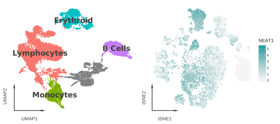
Show code
import cellestial as cl
from ggrust import *
data = cl.datasets.pbmc3k()
dims = gggrid(
[
cl.umap(data, key="cell_type_lvl1", axis_type="arrow", size=1.5, legend_ondata=True)
+ scale_color_hue(),
cl.tsne(
data,
key="NEAT1",
tooltips=["NEAT1", "cell_type_lvl1"],
axis_type="arrow",
size=2,
color_high="#219B9D",
color_low="#f6f6f6",
),
]
) + ggtb(size_zoomin=-1)
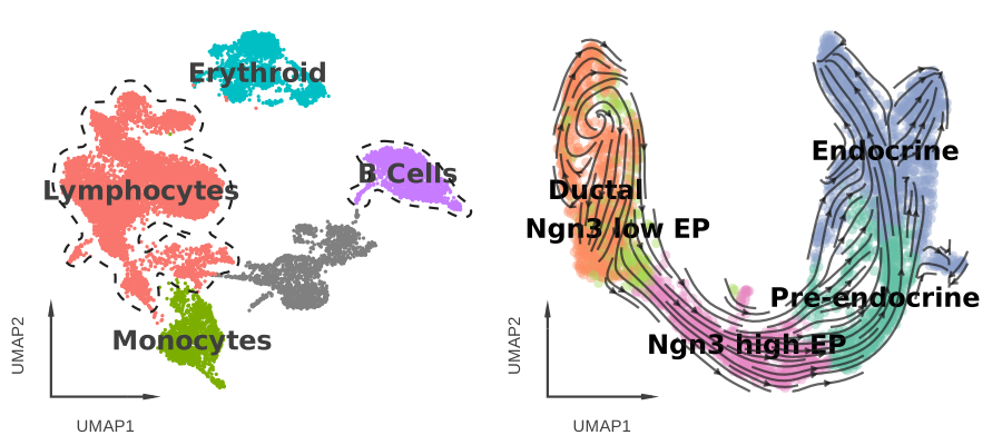
Show code
import cellestial as cl
from ggrust import *
data = cl.datasets.pbmc3k()
data_velocity = cl.datasets.pancreas()
outlined = (
cl.umap(data, key="cell_type_lvl1", axis_type="arrow", size=1.5, legend_ondata=True)
+ scale_color_hue()
+ cl.cluster_outlines(groups=["Lymphocytes", "B Cells"])
)
streamed = (
cl.umap(
data_velocity,
key="clusters_coarse",
axis_type="arrow",
size=4,
alpha=0.4,
)
+ cl.stream()
+ cl.ondata_legend(halo_width=1)
)
layers = gggrid([outlined, streamed]) + ggtb(size_zoomin=-1)
Heatmaps#
Cellestial offers heatmap variants, with built-in dendrogram features.
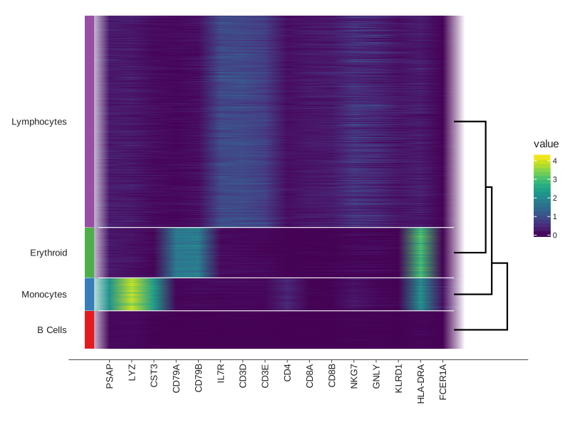
Show code
import cellestial as cl
from ggrust import *
data = cl.datasets.pbmc3k()
markers = [
"PSAP",
"LYZ",
"CST3",
"CD79A",
"CD79B",
"IL7R",
"CD3D",
"CD3E",
"CD4",
"CD8A",
"CD8B",
"NKG7",
"GNLY",
"KLRD1",
"HLA-DRA",
"FCER1A",
]
htmp = (
cl.heatmap(
data,
group_by="cell_type_lvl1",
keys=markers,
geom="raster",
group_lines_size=0.5,
group_lines_color="white",
dendrogram=True,
dendrogram_size=1,
group_bars_labels=True,
group_bars=True,
)
+ scale_fill_viridis()
)
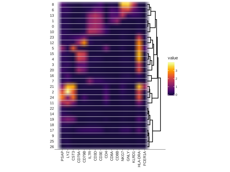
Show code
import cellestial as cl
from ggrust import *
data = cl.datasets.pbmc3k()
markers = [
"PSAP",
"LYZ",
"CST3",
"CD79A",
"CD79B",
"IL7R",
"CD3D",
"CD3E",
"CD4",
"CD8A",
"CD8B",
"NKG7",
"GNLY",
"KLRD1",
"HLA-DRA",
"FCER1A",
]
mtrx = cl.matrixplot(
data,
group_by="leiden",
keys=markers,
group_lines_size=0.5,
group_lines_color="white",
dendrogram=True,
dendrogram_size=1,
) + scale_fill_viridis(option="inferno", begin=0.1)
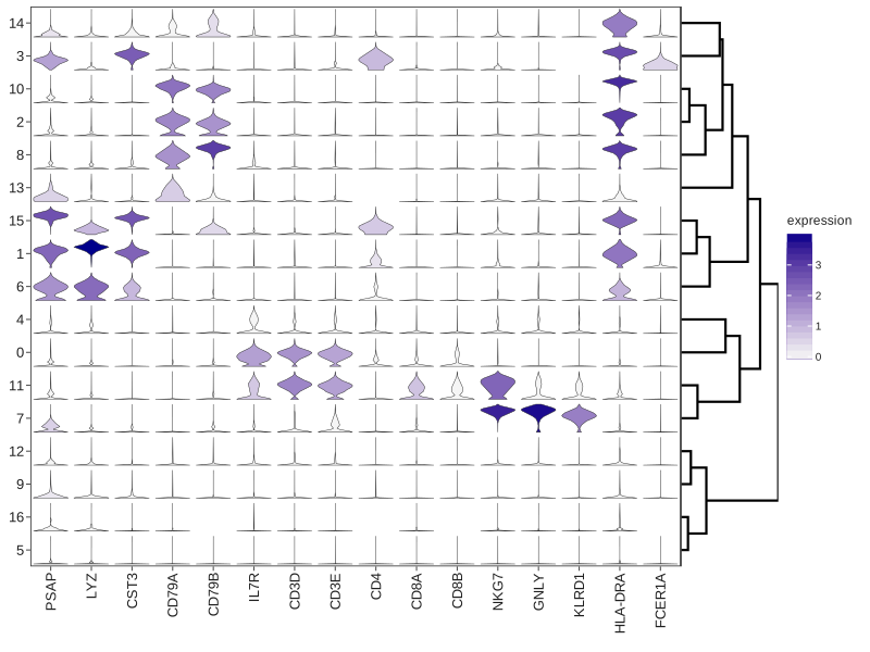
Show code
import cellestial as cl
from ggrust import *
data = cl.datasets.pbmc3k()
markers = [
"PSAP",
"LYZ",
"CST3",
"CD79A",
"CD79B",
"IL7R",
"CD3D",
"CD3E",
"CD4",
"CD8A",
"CD8B",
"NKG7",
"GNLY",
"KLRD1",
"HLA-DRA",
"FCER1A",
]
stck = cl.stacked_violin(
data,
group_by="leiden_res_0.50",
keys=markers,
dendrogram=True,
dendrogram_size=1,
)
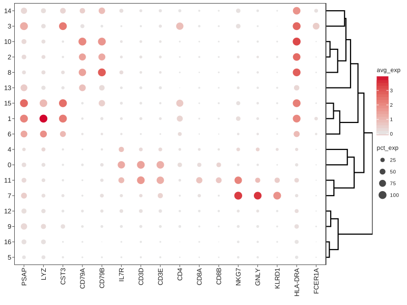
Show code
import cellestial as cl
from ggrust import *
data = cl.datasets.pbmc3k()
markers = [
"PSAP",
"LYZ",
"CST3",
"CD79A",
"CD79B",
"IL7R",
"CD3D",
"CD3E",
"CD4",
"CD8A",
"CD8B",
"NKG7",
"GNLY",
"KLRD1",
"HLA-DRA",
"FCER1A",
]
dtplt = cl.dotplot(
data,
group_by="leiden_res_0.50",
keys=markers,
dendrogram=True,
dendrogram_size=1,
)
Distribution#
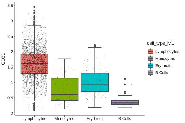
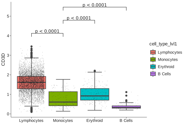
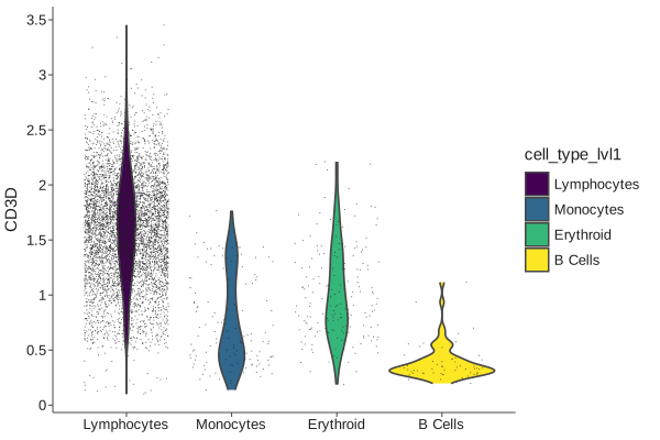
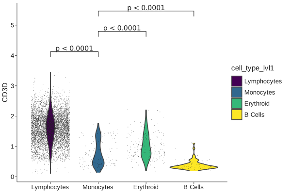
Cellestial comes with distribution (boxplot and violin) plots with built-in statistical analysis.
Show code
import cellestial as cl
from ggrust import *
data = cl.datasets.pbmc3k()
bx = (
cl.boxplot(
data,
key="CD3D",
fill="cell_type_lvl1",
threshold=0.1,
)
+ scale_fill_hue()
)
Show code
import cellestial as cl
from ggrust import *
data = cl.datasets.pbmc3k()
bx = (
cl.boxplot(
data,
key="CD3D",
fill="cell_type_lvl1",
threshold=0.1,
)
+ scale_fill_hue()
)
bx_brckt = bx + cl.bracket(
y_padding=0.2,
label="pvalue",
comparisons=[
("Lymphocytes", "Monocytes"),
("Monocytes", "Erythroid"),
("Monocytes", "B Cells"),
],
)
Show code
import cellestial as cl
from ggrust import *
data = cl.datasets.pbmc3k()
vln = (
cl.violin(
data,
key="CD3D",
fill="cell_type_lvl1",
threshold=0.1,
)
+ scale_fill_viridis()
)
Show code
import cellestial as cl
from ggrust import *
data = cl.datasets.pbmc3k()
vln = (
cl.violin(
data,
key="CD3D",
fill="cell_type_lvl1",
threshold=0.1,
)
+ scale_fill_viridis()
)
vln_brckt = vln + cl.bracket(
y_padding=0.2,
label="pvalue",
comparisons=[
("Lymphocytes", "Monocytes"),
("Monocytes", "Erythroid"),
("Monocytes", "B Cells"),
],
)
Exploratory#
Cellestial ships with quick exploratory plots.
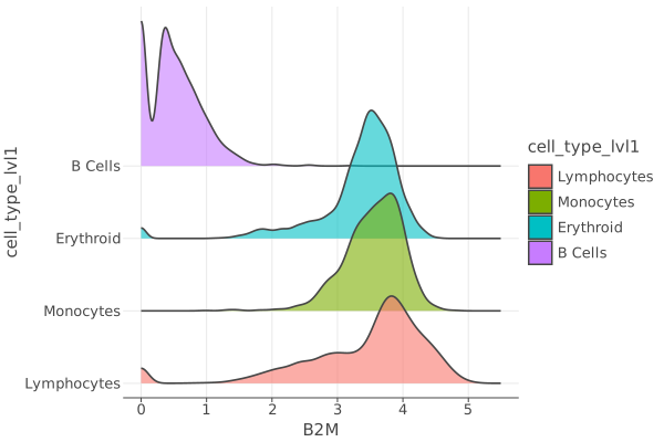
Show code
import cellestial as cl
from ggrust import *
data = cl.datasets.pbmc3k()
rdg = (
cl.ridge(
data,
key="B2M",
alpha=0.6,
group_by="cell_type_lvl1",
)
+ scale_fill_hue()
)
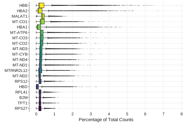
Show code
import cellestial as cl
from ggrust import *
data = cl.datasets.pbmc3k()
hexp = cl.highest_expressed_genes(data, n=20) + scale_fill_viridis()
Documentation#
About ggrust#
Cellestial is built on ggrust, a grammar of graphics
engine written in Rust with a lets-plot compatible Python API.
It renders interactive HTML with tooltips and zooming and panning, and static SVG and PNG.
Layers, scales and themes come from from ggrust import * and compose with +.